On Recurrence Relations And Tail-Call Optimizations

I am currently in the process of working through Functional Programming in Scala by Chisuano and Bjarnason. The book gives a thorough introduction to Functional Programming by showing examples in Scala and providing exercises at various difficulty levels. I also participate regularly in a local Scala enthusiasts meetup where this book is at the core of the syllabus. This is actually how I got started: The meetup is a great way to learn and discuss the material of the book among an interested peer group. You should check out their fork of the code samples and answers at GitHub, since it provides additional summaries and deeper insights into how Scala does the things it does.

Recursion is a topic discussed in chapter 2 of this book. In this short post, I explore this topic from a different angle, discussing how we can get from a mathematical definition of the recurrence to a tail-call-optimized implementation. I will be using the same example, calculating Fibonacci numbers, as in the aforementioned book.

Recursion

In Exercise 2.1 the reader must implement a function that calculates the n-th Fibonacci number. The book provides an informal definition of the Fibonacci sequence: The first two Fibonacci numbers are 0 and 1 and the n-th number is then calculated by adding the previous two Fibonacci numbers. The implemented function must not only be recursive, but also tail-recursive.

Functions that are tail-recursive conclude with the recursive call as their return statement. Thus, a clever compiler can optimize the recursive call and substitute it with an iterative computation process. To make the differences between a recursive and a tail-recursive clear, I will not follow the book and start off with a naive recursive implementation first.

Given the informal definition of the Fibonacci sequence, we can work out the recurrence relation easily.

T(0) = 0
T(1) = 1
T(n) = T(n-1) + T(n-2)

Unlike recursive data structures, where the recursion terminates naturally with the data structure itself (so-called structural recursion), this is a form of generative recursion, where we explicitly have to have a deep understanding of the underlying computation process to provide a termination condition for the recursion. This termination condition is given with T(0) and T(1).

Given the recurrence relation, the naive implementation of the Fibonacci sequence comes down to:

object Exercise_2_1 {

  def fib(n: Int) : Int = {
    if (n == 0) {
      0
    } else if (n == 1) {
      1
    } else {
      fib(n-1) + fib(n-2)
    }
  }
}

Using a test driver for the implementation, we can quickly see that this implementation generates Fibonacci numbers according to their definition.

object Exercise_2_1 {

  [...]
  def main(args: Array[String]) : Unit = {
    (0 to 10).foreach(n => println(fib(n)))
  }
}

However, since the computation is recursive, every recursive call consumes additional space on the call stack. Furthermore, given the definition of the Fibonacci sequence, the same Fibonacci number might be computed multiple times. This is not efficient in terms of execution time and stack space.

Let us see how the computation unfolds. We compute the 5th Fibonacci number, thus calling fib(4) since our implementation of fib is 0-based.

fib(4) = (fib(3) + fib(2))
       = ((fib(2) + fib(1)) + (fib(1) + fib(0)))
       = (((fib(1) + fib(0)) + 1) + (1 + 0))
       = ((1 + 0) + 1) + (1 + 0)
       = (1 + 1) + 1
       = 2 + 1
       = 3

As you can see, for every call to fib, the recursion must unfold as long as it does not hit any of the terminal conditions before the actual value can be computed. Along the way, individual Fibonacci numbers get computed multiple times. While this works for small values of n, it will lead to stack overflows for larger values.

Although elegant in its resemblance to the mathematical definition, one major drawback of our naive implementation is that we do not consider the problem from a holistic point of view. Instead, we divide the given problem into sub-problems and solve those locally. A recursive function that follows this pattern is said to be context-free.

We can work out a smarter solution using so called accumulators. An accumulator collects contextual information along the execution of our computation process. It can be applied to both structural recursive functions and generative recursive functions. By using accumulators, we can turn a recursive function into an equivalent tail-recursive function.

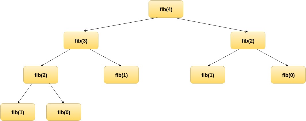
Take a look at the following diagram, which illustrates the same recursive process using a tree-like structure.

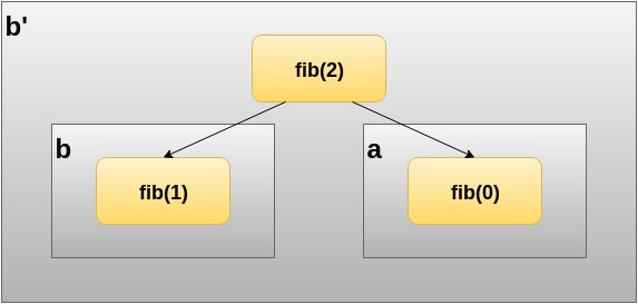
Do you recognize some kind of pattern? The right subtree underneath fib(4) is also part of the left subtree underneath fib(3). Working this from the bottom up, we can derive some simple rules for calculating Fibonacci numbers more efficiently. Take a look at the computational tree for fib(2):

Let us assign variables to the individual calls. Let a = fib(0) = 0 and b = fib(1) = 1, then fib(2) can be expressed in terms of fib(2) = b + a = b', which closely follows the terminal conditions of the recurrence relation.

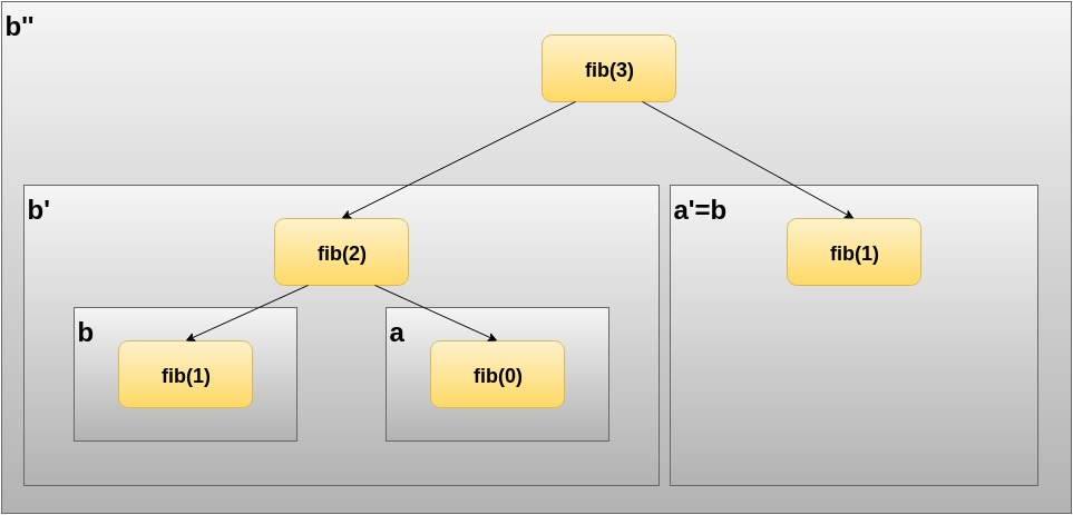
Now that we have an idea of what b' looks like, the question arises: Is there an a' as well? If we would compute the next number, say fib(3), we could re-assign already known values. Take a look at the following illustration.

Computing fib(3) holds fib(3) = fib(2) + fib(1) = b' + a' where a' is simply b which we already know from computing fib(2). It should become clear by now that we require two values as part of our accumulator, which follow the rules underneath when computing the next value recursively:

1. b' = b + a
2. a' = b

We still need a terminal condition. If you look closely at what the accumulator stores for different fib(n), you will notice that variable a always stores the Fibonacci number corresponding to the n-th place in the Fibonacci sequence. Thus, we can use a counter variable n that is initialized with the number we look for and gets decreased by 1 for every recursive call. Our implementation will yield the accumulated value for a if n reaches 0.

Using this, we can implement fib tail-recursively by using an accumulator with the initial values a = 0 and b = 1 (again, following the definition of the recurrence relation).

object Exercise_2_1 {

  def fib(n: Int) : Int = {
    @tailrec
    def f(n: Int, a: Int, b: Int) : Int = {
      if (n == 0)
        a
      else
        f(n-1, b, a+b)
    }
    f(n, 0, 1)
  }
}

Running our test driver shows that the correct numbers are computed. Using the @tailrec annotation shows that we have indeed implemented a tail-recursive function, otherwise the Scala compiler would raise a compilation error.

Let us take a final look at the computation process that this implementation implies. Recall that our naive implementation of fib yields a recursive process:

fib(4) = (fib(3) + fib(2))
       = ((fib(2) + fib(1)) + (fib(1) + fib(0)))
       = (((fib(1) + fib(0)) + 1) + (1 + 0))
       = ((1 + 0) + 1) + (1 + 0)
       = (1 + 1) + 1
       = 2 + 1
       = 3

For our tail-recursive variant of fib, the trace will look like this:

fib(4) = f(4, a, b) = f(4, 0, 1)
       = f(3, 1, 1)
       = f(2, 1, 2)
       = f(1, 2, 3)
       = f(0, 3, 5)
       = 3

Although we do use recursive calls, the computation process is in fact an iterative one. This is actually crucial for understanding why tail-call optimization is possible in the first place! If our implementation of fib would not follow an iterative process, this kind of optimization could not be applied. Since it does, the Scala compiler is able to remove the recursive call and substitute it for a looping construct, thus eliminating unnecessary stack frame allocations which could break our program for large Fibonacci numbers. As a matter of fact, the iterative version comes quite easily to mind once you figured out the tail-recurve version.